Lobachevskii Journal of Mathematics
Vol. 13, 2003, 15 – 24
©M.A.Ignatieva and A.V.Lapin
M.A.Ignatieva and A.V.Lapin
MIXED HYBRID FINITE ELEMENT SCHEME FOR STEFAN
PROBLEM WITH PRESCRIBED CONVECTION
|
________________
2000 Mathematical Subject Classification. Primary. 65M55, 65M60.
Key words and phrases. Mixed hybrid discretization, condensed matrices,
variational inequalities, Stefan problem, iterative methods, spectrally equivalent
preconditioners.
This work was supported by RFBR, project No 01-01-00068.
|
ABSTRACT. We construct a mixed hybrid finite element scheme
of lowest order for the Stefan problem with prescribed convection
and suggest and investigate an iterative method for its solution. In
the iterative method we use a preconditioner constructed by using
”standard” finite element approximation of Laplace operator on a finer
grid.
The proposed approach develops the results of [1], where a spectrally
equivalent preconditioner for the condensed matrix in mixed hybrid finite
element approximation for linear elliptic equation was constructed.
1. Introduction
Stefan problem with prescribed convection serves as a mathematical model for the
heat transfer and solidification process in the metal casting (see [2, 3]).
Commonly used numerical methods of its solving are based on the implicit or
semi-implicit mesh approximations in time variable with lowest order finite element
approximation in space variables [4, 5].
Because in the applied problems both the temperature fields and fluxes are of
practical interest, mixed and mixed hybrid finite element schemes appear as
important method for its numerical solution.
Mixed and mixed hybrid finite element schemes are thoroughly investigated for
the linear boundary-value problems (cf. [6, 7] and bibliography therein), while a few
publications have concern with these methods for nonlinear problems, especially for
free and moving boundary problems. We construct a mixed hybrid finite
element scheme for a Stefan problem which is a case of moving boundary
problem.
The main purpose of the article is to suggest an effective iterative algorithm to
solve this finite element scheme. We construct and investigate an iterative process
with a preconditioner, the rate of convergence of this algorithm does not depend
on the mesh size. On the other hand, the implementation of the iterative
method reduces to the solution of a ”standard” finite-dimensional variational
inequality, which can be made by using any of coordinate or gradient relaxation
methods.
2. Mathematical model
Let Ω ⊂ ℝ2 be a domain with
piecewise smooth boundary ∂Ω = ΓD ∪ ΓN.
We consider the following nonlinear problem: find
(u(x,t),θ(x,t)) such
that
|
∂θ
∂t + v ∂θ
∂x1 − Δu = 0, in Ω,t > 0,
u = z(x,t) on ΓD,t > 0,
∂u
∂n = g(x,t) on ΓN,t > 0,
θ(x,t) ∈ H(u(x,t)) in Ω,t > 0,
θ(x, 0) = θ0(x) in Ω ̄,
| (1) |
where n is the unit vector
of outward normal, v = const > 0,
z, g and
θ0
are given functions. We consider the case when the graph of
H : ℝ1 → ℝ1
monotonically increases and contains a vertical segment and suppose that the function
H has a single values
at points on ΓD.
Problem (1) can serve as a simplified model of continuous casting process, where
u is the temperature of
casting metal, θ(u) is the
enthalpy function and v
is the casting speed in x1
direction. The enthalpy function has a mentioned above property for example in the
case of copper casting.
The existence and uniqueness of a weak solution for problem (1) are studied in
[8, 9].
3. Semi-discretization
First, we introduce the semi-discretization of problem (1) using the
characteristics of the first order differential operator and constant steps
τ in time. Namely,
if (x1,x2,t) is the point at
the time level t
we use the following approximation:
∂
∂t + v ∂
∂x1H ≈ 1
τ H(x1,x2,t) − H(x˜1,x2,t − τ) ,x˜1 = x1 − vτ.
If x1 − vτ < 0 then
we put x˜1 = 0.
After semi-discretization problem (1) on each time level can be formally written
in the pointwise form as
|
−Δu + Pu ∋ f in Ω,
u = z on ΓD,
∂u
∂n = g on ΓN,
| (2) |
where Pu = H(u)∕τ
is the multivalued maximal monotone nonlinear operator and the right-hand side
f = H˜(u)∕τ also
arises due to semi-discretization.
Because of maximal monotonicity of function
H and the
property Dom(H)
= ℝ the
operator Pu
is the subdifferential of convex continuous function
ϕ(u). The
weak formulation of problem (2) can be written in the form of variational inequality:
find u(x) ∈ H1(Ω),
u(x) = z(x) on
ΓD such
that
|
∫
Ω∇u∇(q − u)dx + ϕ(q) − ϕ(u) ≥∫
Ωf(q − u)dx + ∫
ΓNg(q − u)dΓ
| (3) |
∀q ∈ H1(Ω),
q(x) = z(x) on
ΓD .
It is well known that (3) has a unique solution [10].
4. Mixed hybrid formulation of the problem
Now, let v = ∇u
be so called flux function, then we get the following mixed formulation of (2):
|
v −∇u = 0 in Ω,
div v − Pu ∋−f in Ω,
u = z on ΓD,
v ⋅ n = g on ΓN.
| (4) |
Let H(div, Ω) = {w ∈ L2(Ω)n : div w ∈ L
2(Ω)} with
the norm ∥w∥2 = ∫
Ω(∣w∣2 + ∣ div w∣2)dx,
H(div, Ω) = {w ∈ H(div, Ω) : w ⋅ n ∈ L2(∂Ω)} with the
norm ∥w∥H2 = ∥w∥2 + ∫
∂Ω(w ⋅ n)2dΓ and
subspaces HN(div, Ω) = {w ∈H(div, Ω) : w ⋅n̄ = g a. e. on ΓN},
HN0(div, Ω) = {w ∈H(div, Ω) : w ⋅ n = 0 a. e. on Γ
N}.
Now by a weak solution of problem (4) we mean a triple
(u,v,σ) ∈ L2(Ω) ×HN × L2(Ω), such
that
|
∫
Ωv ⋅ wdx + ∫
Ωu div wdx −∫
ΓDz(w ⋅ n)dΓ = 0∀w ∈HN0,
∫
Ω div vqdx −∫
Ωσ(x)qdx = −∫
Ωfqdx∀q ∈ L2(Ω),
σ(x) ∈ Pu(x) for a. e. x ∈ Ω.
| (5) |
Note, that by construction if u
is solution of (5) then (u,∇u,σ)
is a solution of problem (5).
Let Ω ̄ = ⋃
i=1mē
i be a partitioning of the
domain into m nonoverlapping
subdomains, where ei
has a piecewise smooth boundary. Hereafter we suppose that the parts
ΓD and
ΓN of the boundary
∂Ω are composed by the
whole sides ∂ei. The common
sides of elements ei
and ej we
denote by Γij,
where i≠j,
i, j = 1,m¯. We suppose
that ∂Ω consists of
s segments, which
we denote as Γ1,…, Γs. Let
the intersections ∂ei
with Γj,j = 1,s¯ be
denoted by Γi,m+j,
i = 1,m¯,
j = 1,s¯ and
let Γi,m+j
for j = 1,s1¯,
s1 < s compose
ΓN , while
Γi,m+k,
i = 1,m¯,
k = s1 + 1,s¯ compose
ΓD .
Let further v = (v1,…,vm),
u = (u1,…,um). Then
system (4) can be written in the following form
|
vi −∇ui = 0, div vi − σi = −fi,σi ∈ Pui in ei,
ui − uj = 0,vi ⋅ nij − vj ⋅ nij = 0 on Γij,i,j = 1,m¯,
ui = z on Γi,m+k,k = s1 + 1,s¯,
vi ⋅ ni = g on Γi,m+j,j = 1,s1¯,
| (6) |
where ni is the outward
normal vector to ∂ei
and nij is the unit
normal vector to Γij
directed from ei
to ej.
Let us note that in semi-discretized problem the flux function
v ⋅ n is continuous
in Ω
though in initial differential problem flux may have a jump.
On the basis of (6) we define a weak mixed hybrid formulation of problem (2). Let
U = ∏
1≤i≤mL2(ei),V = ∏
1≤i≤mH(div,ei) and
Λ = ∏
i>jL2(Γij). We introduce the
bilinear forms M : V × V → ℝ,
B : U × V → ℝ,
C : Λ × V → ℝ and
D : U × U → ℝ by
the following equalities
M(v,w) = ∑
i=1m ∫
eivi ⋅ widx,B(u,w) = ∑
i=1m ∫
eiui div widx,
C(λ,w) = ∑
i=1m ∑
j=i+1m ∫
Γijλij(wj−wi)⋅nijdΓ−∑
j=1s1
∫
Γi,m+jλi,m+j(wi⋅ni,m+j)dΓ,
D(q,σ) = ∑
i=1m ∫
eiσiqidx
and linear functionals
F(q) = ∑
i=1m ∫
eifqidx,ℓ(μ) = ∑
i=1m ∑
j=1s1
∫
Γi,m+jgμi,m+jdΓ,
r(w) = ∑
i=1m ∑
k=s1+1s ∫
Γi,m+kz(wi ⋅ ni)dΓ.
The weak mixed hybrid formulation is as follows: find
(u,v,λ,σ) ∈ U × V × Λ × U such
that
|
M(v,w) + B(u,w) + C(λ,w) = r(w)∀w ∈ V,
B(q,v) + D(q,σ) = −F(q)∀q ∈ U,
C(μ,v) = −ℓ(μ)∀μ ∈ Λ,
σ(u) ∈P̄u,
| (7) |
where P̄u = (H(u1)∕τ,…,H(um)∕τ)
for u ∈ U.
Proposition 1. The problems (3) and (7) are equivalent in the following
sense:
if u
is the solution of (3), then (u,v,λ,σ)
with ui = uei
- restriction of u
to ei,
vi = ∇ui
a. e. in ei,
λij = ui
a. e. on Γij
and σ ∈P̄(u)
is the solution of (7);
backwards, if
(u,v,λ,σ)
is the solution of problem (7), then the function
u : uei = ui
is a solution to problem (3).
5. Approximation
Let further Ω be a
polygonal domain and τh = {e1,e2,…,em}
be its conforming triangulation [11]. We assume that all
ei are
convex polygons.
Let Uh,V h
and Λh
be finite element subspaces of the corresponding spaces
Uh = ∏
1≤i≤mUih,V h = ∏
1≤i≤mV ih
and refer to Λh
as the space of vector-functions with constant components. Here
V ih is a finite dimensional
subspace in H(div,ei) of
dimension ni consisting of
vector-functions vi ∈H(div,ei) such
that vi ⋅ nij is a constant on the
corresponding interface Γij
and Uih is a
subspace of U
consisting of vector-functions such that each its coordinate is a constant on each subdomain
ei . The value of
ni is equal to the total number
of interfaces Γij belonging
to the boundary of ei,
i = 1,m¯. Thus, the
dimension of V h is
equal to n̂ = ∑
i=1mn
i, the
dimension of Uh is
equal to m, and
the dimension of Λh
is equal to ň
where ň
is the total number of interfaces.
The finite element approximation of (7) reads as follows: find
(uh ,vh,
λh ,σh) ∈ Uh × V h × Λh × Uh
satisfying the following relations:
|
M(vh,w) + B(uh,w) + C(λh,w) = r(w)∀w ∈ V h,
B(q,vh) + D(q,σ(uh)) = −F(q)∀q ∈ Uh,
C(μ,vh) = −ℓ(μ)∀μ ∈ Λh,
σh ∈P̄u.
| (8) |
Let now vij be the degrees of
freedom for vector-function vih,
associated with Γij,
ui be the degrees of
freedom for the function uh,
associated with ei, and
λij be the degrees of freedom
for λh, associated with
Γij ,j > i. The algebraic formulation
of (8) is: to find (v̄,ū,λ̄,σ̄)
such that
|
M̂(v̄,w̄) + B̂(ū,w̄) + Ĉ(λ̄,w̄) = r̂(w̄),
B̂(q̄,v̄) + D̂(q̄,σ(ū)) = −F̂(q̄),
Ĉ(μ̄,v̄) = −ℓ̂(μ̄),
σ̄ ∈P̄ū,
| (9) |
∀(w̄,q̄,μ̄) ∈ ℝn̂ × ℝm × ℝň.
Here
M̂(v̄,w̄) = ∑
i=1m(M
iv̄i,w̄i),v̄i,wi ∈ ℝni
,
B̂(ū,w̄) = ∑
i=1mu
i(−∑
j=1i−1w
ij∣Γij∣ + ∑
j=i+1m+sw
ij∣Γij∣),
Ĉ(λ̄,w̄) = ∑
i=1m(∑
j=i+1mλ
ij(wji−wij)∣Γij∣−∑
i=1s1
λi,m+jwi,m+j∣Γi,m+j∣),
D̂(q̄,σ̄) = ∑
i=1mσ
iqimes(ei)
are the bilinear forms on ℝn̂ × ℝn̂,
ℝm × ℝn̂,
ℝň × ℝn̂ and
ℝm × ℝn̂,
respectively, and
r̂(w̄) = ∑
i=1m ∑
j=s1+1sz
i(wi ⋅ ni)dΓ,∫
Γi,m+jzdΓ,i = 1,m¯,j = s1 + 1,s¯,
F̂(q̄) = ∑
i=1mf
iqi,fi = ∫
eifdx,i = 1,m¯,
ℓ̂(μ̄) = ∑
i=1m(∑
j=1s1
gijμi,m+j),gij = ∫
Γi,m+jgdΓ,i = 1,m¯,j = 1,s1¯
are linear forms defined on ℝň,
ℝm and
ℝň .
The entries mk,l(i) of matrices
Mi are defined by the
standard way using the L2(ei)
scalar products of the nodal basis functions of the subspaces
V ih.
In matrix-vector form problem (9) can be written as follows:
|
A v̄
ū
λ̄ + 0
−P̄(ū)
0 ∋ r̄
−f̄
−ḡ ,A = MBT CT
B 0 0
C 0 0 .
| (10) |
We rewrite the system as
|
Mv̄ + BT ū + CT λ̄ = r̄,
Bv̄ −P̄ū ∋−f̄,
Cv̄ = −ḡ
| (11) |
and eliminate v̄
from the system. After that we obtain a reduced system which can be written in
block form by
BM−1BT BM−1CT
CM−1BT CM−1CT
ū
λ̄
+ P̄ū
0 ∋ f + BM−1r̄
g + CM−1r̄
.
Using notations
S = BM−1BT BM−1CT
CM−1BT CM−1CT
,μ = ū
λ̄
,
F = f + BM−1r̄
g + CM−1r̄
,P˜ = P̄0
0 0
,
we finally obtain the following finite-dimensional problem:
Note that Schur complement matrix S
is a symmetric and positive definite matrix [1], while
P ˜ is a
maximal monotone operator. Owing to this fact problem (12) has a unique solution,
whence problem (11) has also a unique solution.
6. Iterative method
For the sake of simplicity we analyze only the case of rectangular meshes. We suppose that
Ω is the unit square and
construct mesh with step h
in both directions which defines the partitioning of
Ω into
elements ei.
To obtain preconditioner for (12) we construct finer grid in
Ω with the step
h∕2. We denote by
τh∕2 the new partitioning
of Ω. Let further
W h∕2 be the piecewise finite
element subspace of H1(Ω)
and A
be the stiffness matrix, corresponding to the approximation in this
subspace of Laplace operator with Dirichlet boundary conditions on
ΓD . Let the
nodes of τh∕2
consist of two groups: the first group contains the nodes of
τh , while
the second one contains all others (called by the fictitious ones). Then matrix
A can
be represented in the corresponding block form:
A = A11A12
A21A22 .
It is shown in [1] that the operator S
is spectrally equivalent to the Schur complement
SA :
SA = A11 −A12A22−1A
21
with constants of equivalence which do not depend on mesh size:
α(SAμ,μ) ≤ (Sμ,μ) ≤ β(SAμ,μ)∀μ.
In the case under consideration we get
α = 1,
β = 6.
This observation allows us to use the matrix
SA as a
preconditioner in iterative process for solving (12):
|
SAμn+1 − μn
τ + Sμn + P˜μn+1 ∋ F.
| (13) |
The following statement is valid.
Proposition 2. The iterative method (13) converges for any
τ ∈ (0, 2∕β)
and for
τ = 2∕(α + β)
the following estimate holds:
(SA(μn+1 − μ),μn+1 − μ)1∕2 ≤ β − α
β + α(SA(μn − μ),μn − μ)1∕2.
To avoid the explicit calculation of SA
on each step of process (13) we use the following trick. We complete the system (12)
by the equations in fictitious nodes, so that the algebraic size of resulting
system
Sμ + P˜μ ∋ F,
0 = 0
is equal to number of fine grid nodes. After we write iterative process with operator
A
as a preconditioner for this system using block representation of
A:
|
A11μn+1 − μn
τ + A12μ˜n+1 −μ˜n
τ + Sμn + P˜μn+1 ∋ F,
A21μn+1 − μn
τ + A22μ˜n+1 −μ˜n
τ + 0 = 0,
| (14) |
where μ˜
are fictitious components. Eliminating from the second equation fictitious values we
can verify that it is an equivalent form of process (13) for solving (12) with
SA as
preconditioner.
For a fixed n
problem (14) is the finite element variational inequality with positive definite and symmetric
matrix A,
so, it can be solved, for example, by using any coordinate relaxation or gradient
relaxation method.
On each step of constructed method we need to calculate
F − Sμ. It is
easy to do if we take into account the identity
F−Sμn = Bv̄n
Cv̄n
with v̄n = M−1(r̄ − BT ūn − CT λ̄n).
Thus, to solve (14) we get the the following
Algorithm
- Define μ0 = (ū0,λ̄0).
- For n ≥ 0
on each element ei
calculate v̄n
by formula
v̄in = M
i−1(r̄
i − BiT ū
in − CT λ̄
in).
- Calculate μn+1 = (ūn+1,λ̄n+1)
by solving (14).
- n := n + 1
goto step 2.
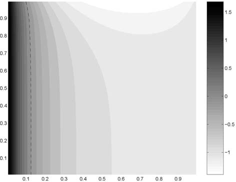
7. Numerical results
In numerical test we take Ω = (0, 1) × (0, 1),
ΓD = {(x1,x2) ∈ ∂Ω : x2 = 0}∪{(x1,x2) ∈ ∂Ω : x2 = 1},
ΓN = ∂Ω ∖ ΓD.
We solve problem in time interval [0,1] using constant time step
τ = 0.05
and various grids in space to compare number of iterations. As
H we
take the function
H(u) = 0.5u if u < 0,
0, 1 if u = 0,
u + 1 if u > 0.
On the top of square Ω
we put g = −3
in the boundary condition, on bottom we use value
g = 0, on the left side
z = 2, and on the right
side z = −1. As initial
condition we take u0 = −1.
To solve inequality with matrix A
on each step of iterative process (14) we use SOR-method, the stopping criterion was
∥μk+1 − μk∥≤ 10−13 and the stopping criterion
of outer process was ∥μn+1 − μn∥≤ 10−12.
As iterative parameter in outer process we take
τ = 2∕7,
which we get using estimates of equivalence of matrices
S and
SA .
In the second column of table 1 we show the number of iteration which we need
to solve problem on the first time level (on the next levels the number of
iterations becomes smaller) and in the third column – the total number of
iteration, which is equal to the sum of iterations on all time steps. From the
table we can see that the number of iterations does not depend on mesh
size.
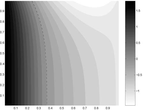
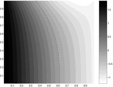
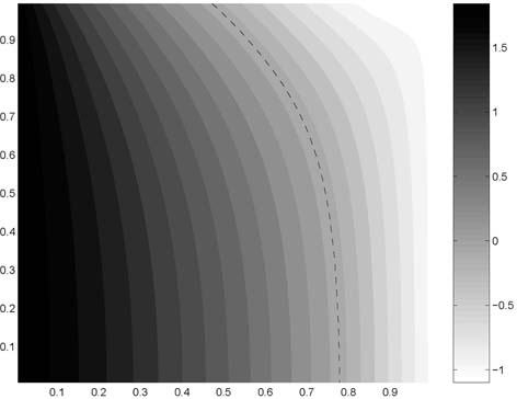
On the figures we show temperature distributions at several time levels.
|
|
| | | | | | | | | | | Grid size | Iter 1 | Total Iter |
|
|
| | 11 × 11 | 81 | 1195 |
| 21 × 21 | 82 | 1183 |
| 41 × 41 | 83 | 1189 |
| 81 × 81 | 83 | 1189 |
| 161 × 161 | 83 | 1171 |
|
|
| | |
| Table 1: | Number of iterations |
|
References
[1] Kuznetsov Yu. A. Spectrally equivalent preconditioners for mixed hybrid discretizations
of diffusion equations on distorted meshes // J. Numer. Math. – 2003. – V. 11 – P.61–74.
[2] Louhenkilpi S., Laitinen E., Nieminen R. Real-time simulation of heat transfer in
continuous casting//Metallurgical Trans. B. – 24B. – 1996. – P. 685–693.
[3] Ma¨kela¨
M., Ma¨nnikko¨
T., Schramm H. Applications of nonsmooth optimization methods to continuous casting
of steel//Math.Ins., Univ. Bayreuth. – Rep. No 421 – 1993. – 24 p.
[4] Chen Z., Jiang L. Approximation of a two phase continuous casting problem // J. Part.
Diff. Equations. – 1998. – V. 11. – P. 59–72.
[5] Laitinen E., Lapin A., Pieska¨
J. Mesh approximation and iterative solution of the
continuous casting problem // in: ENUMATH 99. Ed. by P.
Neittaanma¨ki,
T. Tiihonean and P. Tarvainen. World Scientific, Singapore. – 2000. – P. 601–617.
[6] Brezzi F., Fortin M. Mixed and hybrid finite element methods. – New-York: Springer
Verlag, 1991.
[7] Roberts J.E., Thomas J.M. Mixed and hybrid methods//Numer. Anal. – 1991. – V. II. –
P. 523–639.
[8] Rodrigues J.F., Yi F. On a two-phase continuous casting Stefan problem with nonlinear
flux//Euro. J. Appl. Math. – 1990. – No 1. – P. 259-278.
[9] Rodrigues J.F. Variational methods in the Stefan problem//Lect. notes in math. – 1994.
– Springer Verlag. – P. 149–212.
[10] Lions J.L. Quelques méthodes de résolution des problèmes aux limites non linéaires.
– Paris: Dunod Gauthier-Villars, 1969.
[11] Ciarlet P.G., Lions J.L. Handbook of numerical Analysis. Volume II: Finite element
methods (Part I). – Amsterdam: Elsevier, 1991. – 928 p.
KAZAN STATE UNIVERSITY, RUSSIA
E-mail address: alapin@ksu.ru
Received October 15, 2003